Manual

Editing Interference Velocity Data:

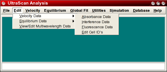
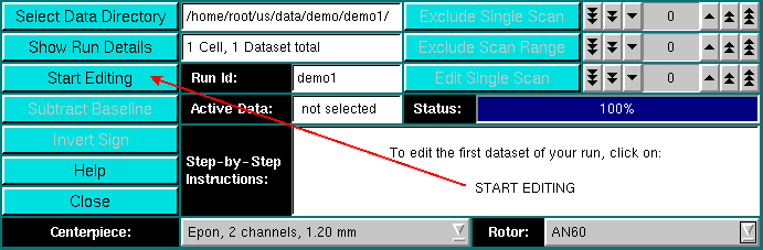
All experimental velocity data aquired on the XL-A require substantial editing and preliminary diagnostics before the data can be successfully analyzed with various analysis methods. UltraScan assists you in this process by handling most essential diagnostics and editing steps automatically, but permits you to intervene, where necessary. Editing is started by selecting

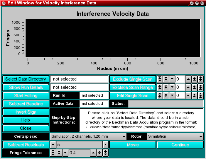
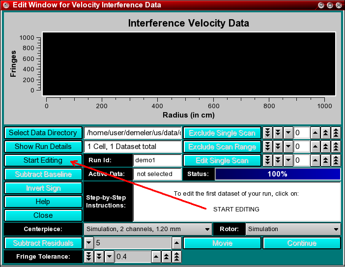
from the main menu of UltraScan. This will bring up the editing window with the plot area and the control panel.

At the bottom of the control panel is a "Wizard" that provides step-by-step instructions to guide you through the multi-step process of velocity data editing. Refer to it to determine which action is required next.

Step 1: Select a data directory that contains the data files acquired by the Beckman data acquisition program by clicking on the "Select Data Directory button on the upper left. Such a directory can generally be found as a subdirectory of the Beckman data acquisition software. The default installation for the Beckman software is C:\XLAWIN (under Windows). Under Unix, the drive with Windows 3.11/95 will generally be mounted under the /dosc or /dos directory. You can always set the desired default location in the configuration panel so you can avoid lengthy directory traversals to find the desired location quickly.

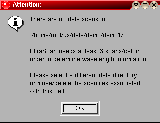
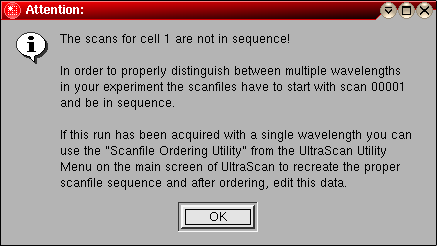
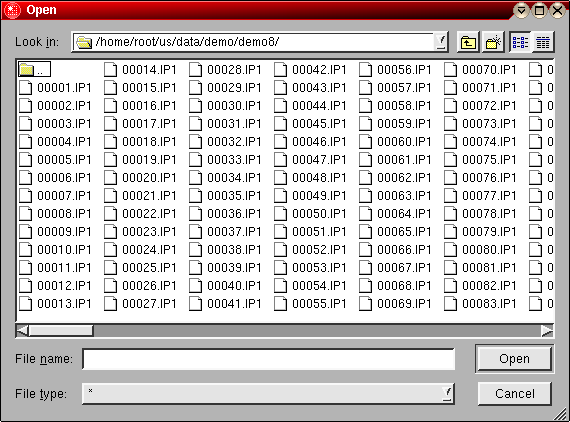
The experimental data will then be located in a subdirectory of the form mmddyy/hhmmss (month/day/year/hour/min/sec), identifying the date and time on which data acquisition commenced for a particular run. A file dialog will allow you to specify the desired directory. If the directory contains files of the type 00001.ip1, 00002.ip1, ..., etc., then it is a proper data directory. If the program cannot find enough scans in the selected directory, a warning message will be printed on the screen.

Note:
Data directories retrieved from the database contain an additional file called "db_info.dat" which contains database index information that is automatically included in the edited data. The file is parsed during editing and parameters such as run identification, celltype, centerpiece type, rotor, buffer corrections, etc. are included in the edited data and later available during analysis.

Once you have navigated through the directory tree to the desired data directory, simply press the OK button (there is no need to highlight or individually select scans in the directory, specifying the directory itself is sufficient). Next, the program will load the data in this directory and determine a number of important diagnostics from the scan files present in this directory:

1. The number and position of cells that were scanned in this run. If not enough datapoints are found in the selected directory, a warning message will be printed. If the sequence of the scan files is out of order, a warning message will be shown. If this message shows up, and you acquired the data at a single wavelengths, you can rescue your data by rebuilding the data sequence with the Scanfile Reordering Utility.
2. The number of scans that were measured for each cell and the wavelength of the laser
3. The average temperature over the entire run
4. The program will determine if the temperature varied for more than a pre-set tolerance value over the course of the run and warn the user if the tolerance was exceeded. In this case, a warning message is printed forcing the user to acknowledge the diagnostic before editing can resume.
5. The time correction in minutes and seconds accounting for the rotor acceleration period at the beginning of the run. Due to the near linear acceleration of the XL-A, this number will typically be about half of the time it took to reach final rotor speed. If you acquired your velocity data with an older version of the Beckman data acquisition program that failed to correctly record the times of the scans to file, you will get a warning message. In this case you may want to turn on the compensation switch in the configuration panel. This message can also be generated when there were more than usual initial scans made at a low speed. In that case it is safe to ignore the warning, since the delay is real. (Loading equilibrium data will often generate this message as well, of course, you shouldn't attempt to edit equilibrium data with this method.)
6. The length (duration) of the entire run in hours and minutes
7. The rotor speed at which the measurements were made
8. The identifications for each cell that were entered at the begin of the run.

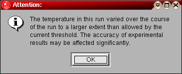
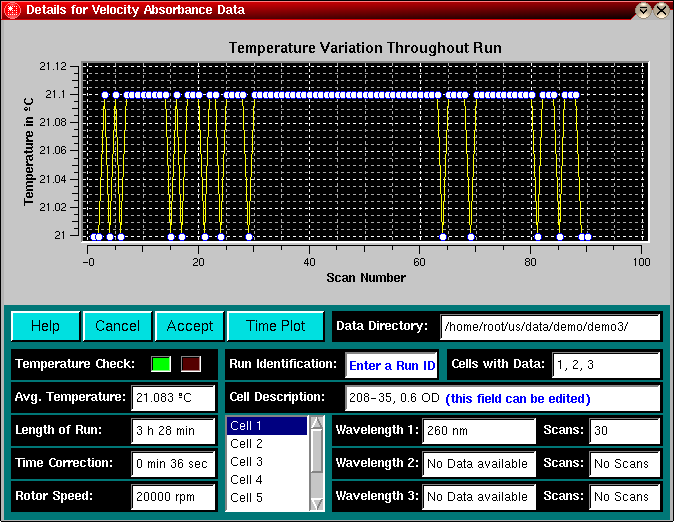
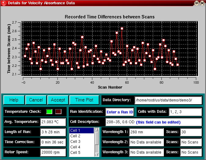
The status bar will keep the user informed about the progress of the diagnostics. The length of time required to complete these diagnostics will depend on the number of files in the directory that have to be analyzed. Once the diagnostics are completed, the diagnostics window will be displayed that shows the details of the selected run. The top panel of the "Run Detail" Window will provide you with a profile of the temperature variation over the course of the run. Shown is the temperature value of each scan in the experiment. Ideally, the temperature should not vary more that a few tenth of a degree over the course of the run. If the temperature varies more than a pre-set tolerance value, the "Temperature Check" field will show a red flashing LCD, otherwise a continuous green LCD.

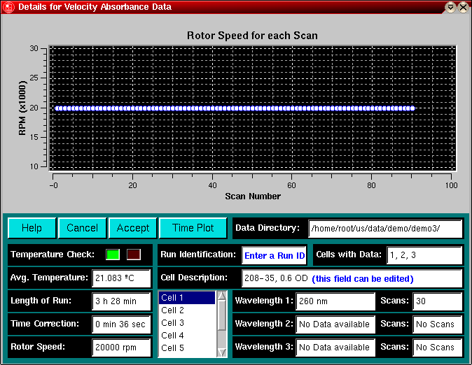
Clicking on the "Time Plot" button will present you with a plot of the time differences between scans. The "Time Plot" button will then change to a "Speed Plot" button. Clicking on the "Speed Plot" button will then show you a plot of the speed at which each scan was recorded. Finally, you can recall the temperature plot by clicking on the "Temp. Plot" button, and cycle through the different plots by repeatedly clicking on the same button.

The purpose of this window is to facilitate the identification of experiments from the rather cryptic information provided by the file- and directory names created by the Beckman data acquisition software. Information about various cells available for a particular run can be obtained by selecting the appropriate cells in the listbox (UltraScan allows for up to 8 cells to accommodate experiments performed with the 8-hole rotor AN-50 Ti, and allows for an unlimited number of scans to be analyzed for each dataset. The cell description will be updated for each cell that is selected in the listbox. If the description for a particular cell was not sufficient, it can now be updated and edited to accommodate changes. After editing is complete, you can also edit the description of each cell with the Cell ID Editing Utility for the edited data.

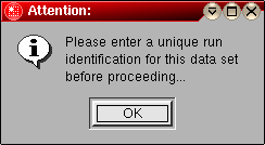
Step 2: Before editing of the data can proceed, a unique run identification needs to be entered in the box labeled "Run Identification". This run identification should not contain any spaces and should help the user in identifying the run by name. Spaces can be replaced by underscores. Please note that unlike under Microsoft Windows, file names will follow Unix naming conventions, which are case sensitive. For example, a run identification such as "Chromatin_pH8" is distinct from "chromatin_ph8". A practical way of naming runs is to use the logbook number of the run, and to append a "v" for velocity-, or an "e" for equilibrium runs. If the data was retrieved from the database, the run identification will be filled in automatically.

If you change your mind and do not want to edit this data, you can cancel the editing process at this point by clicking on "Cancel" and you can then select a different directory instead. However, if you do want to proceed, click on "Accept". If you forgot to enter a unique run identification, you will be reminded by an error message.

Step 3: Make sure that the cell descriptions are correct and adequate to identify the contents of each cell that contains data. If not, you can now edit the description for each cell by modifying the string in the editable text box. After entering a unique run identification, the window will close and you will return to the main editing window. The control panel will now show all fields updated with the proper information obtained during the diagnostics. If the data directory was retrieved from the database, the run identification is automatically set and all cell and centerpiece parameters should be automatically set to their proper values. Otherwise, adjust the centerpiece, cell and rotor settings now. Some data analysis methods rely on the geometry information included in these definitions.

The number of editable datasets will be displayed in the "Run Detail" box. A dataset is the collection of scans acquired for a particular wavelength and a single cell. To load the first dataset for editing, click on the Start Editing button, which is now highlighted. All scans will then load into the editing plot window, and the status bar indicates the progress of data loading.

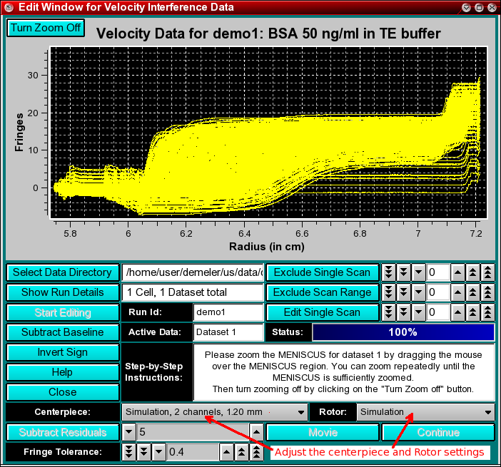
Step 4: After loading is completed, the data will be displayed in the editing window. Review the settings for rotor selection and centerpiece type, and adjust if needed. The selection of these items determines the method of editing as well as the cell dimensions for the finite element fit. If the data was loaded from a directory that was retrieved from the database, these settings should already be adjusted to their appropriate values.

In case the sample and reference channels were reversed during loading, you can click on the "Invert Sign" button to flip the data back into a standard display mode.

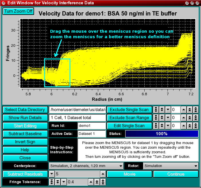
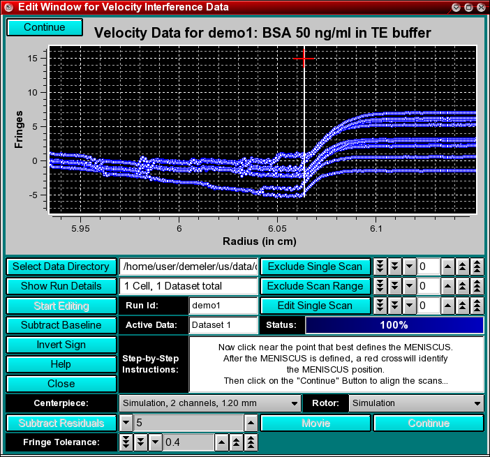
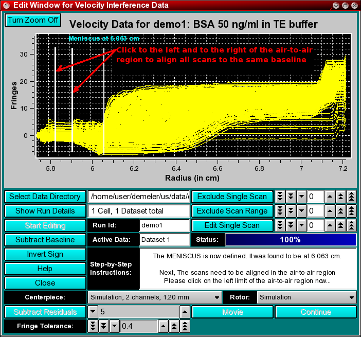
Next, you will have to define the meniscus position. Interference data generally do not show a well defined meniscus in the image of the data, therefore the exact meniscus position cannot easily be determined automatically. Drag the mouse over the area that contains the meniscus in order to zoom the region. Only the first 8 scans of the run will be shown for clarity. You can increase the zoom level by repeatedly dragging the mouse over a smaller and smaller plot region. Once you reached the desired zoom level, click on the "Turn Zoom Off" button and click at the appropriate radial position in the plot that best identifies the position of the meniscus. A vertical bar will be drawn at the position of the mouseclick, and crosshairs identifying the closest radial datapoint position will be displayed. Now click on the "Continue" button. The entire data will now be shown with the meniscus position marked by a vertical bar.

Step 5: Now you will have to correct the baseline interference of each scan by aligning all scans in the air-to-air region. Select a point left and right of an area suitable for averaging in the air-to-air region. Two vertical bars will be drawn to identify the limits. The air-to-air region can be found between the start of the cell and the first meniscus (in most cases the meniscus from the buffer). After defining the right limit, the program will automatically align all scans along the same baseline level, and you should get a picture similar to this one.

Important Note: In order to obtain an air-to-air region it is necessary that both reference and sample channel contain a little airspace. Since buffers contain salts and other refracting substances, it is important that the menisci are at the same position in both channels, since such compounds will also form a concentration gradient during sedimentation and if the gradients are different on both sides, systematic error will be introduced into the experimental data.

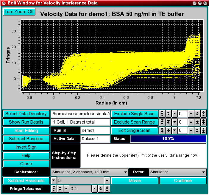
Step 6: The next step requires that the data limits are chosen. Those are the limits between which the data contains useful information for data analysis. This region should exclude the meniscus and the bottom of the cell.

Important Note: You should collect interference data from the very beginning of the run, when hardly any material has sedimented. Such early data will have very little curvature or boundary information, since the concentration distribution is still homogeneous throughout the cell. Such early data should therefore be essentially horizontal throughout the cell. Since interference data suffer from time invariant noise from refractive index heterogeneities in the cell windows, all such time invariant noise patterns will be in the initial scan as well. Since the theoretical pattern should be completely horizontal, all deviations from a horizontal line will be due to the time invariant refractive index heterogeneities in the windows. When picking the left limit, try to select the limit at such a point that the first scan is completely horizontal, i.e., without starting to show a moving boundary. By selecting the cropping limits such that any early boundary formation is excluded, it is possible to use the first scan as a "baseline" and subtract it from all other scans to effectively remove the refractive index patterns from all other scans. Therefore, it is necessary to start collecting data as early as possible in the run in all interference experiments to make sure such a horizontal scan is available for baseline subtraction.

First, the left limit is defined by clicking the mouse at a position near the top of the sample solution column. Next, define the right limit of the useful data by clicking near the bottom of the cell.

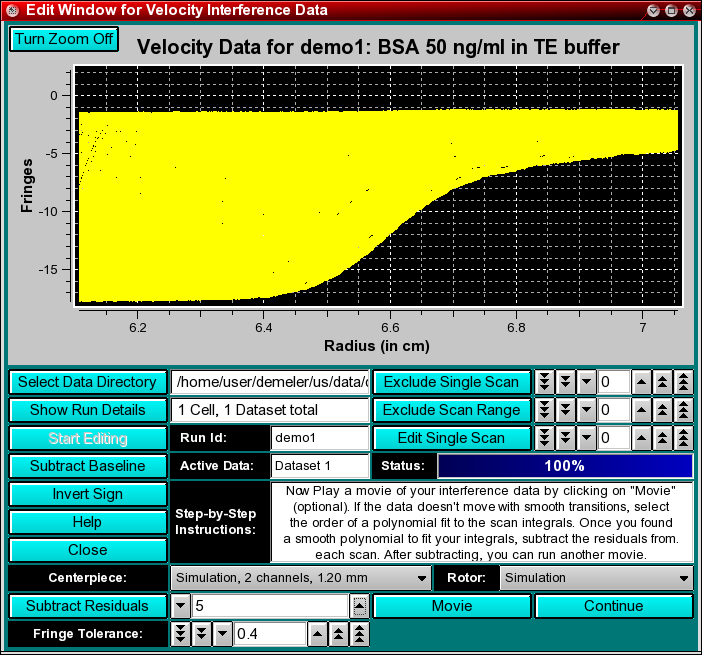
Step 7: As soon as the right limit has been selected, the data will be cropped between the limits and rescaled to the new limits, and all the extraneous datapoints will be discarded. In addition, the software will automatically correct for integral fringe jumps present in the data and align all scans to the fringe integral of the first scan. This absolute alignement is arbitrary and can be different from run to run.

Step 8 (optional): At times, when data are very noisy, the algorithm may have trouble correctly identifying the fringe offsets. This is done by integrating the scans and ordering scans according to integral values; the highest integral should be the first scan, and each subsequent scan should have some lower integral value. Integral offsets are adjusted such that this order is maintained. On occasion, the offsets are distorted by noise, and the integral values aren't really integral. In such cases, adding a fudge factor to all integral can solve the problem. This is determined visually by adjusting the "Fringe Tolerance" value. If the fringe offsets do not follow a smooth curve, adjust this tolerance until most of the scans have reasonable fringe offset corrections. This may require increasing or decreasing the fringe tolerance. The default value should work unchanged for most cases.

Step 9 (optional): Now you will have the opportunity to exclude and edit scans. To edit spikes and other imperfections in the data, follow the protocol outlined here.

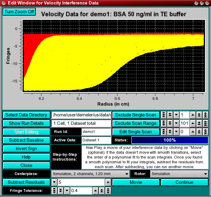
Step 10 (optional): Next, you may want to exclude a number of scans from the run. While not strictly necessary at this point, you can exclude a single scan by clicking on the Exclude Single Scan or a range of scans by clicking on "Exclude Scan Range", after setting the scan number in the counter. Arrow buttons move in steps of 1, 10, or 100, depending on how many arrows are shown on the button (1, 2 or 3). As you select scans, the about to be excluded scans will be highlighted in red. After clicking on one of the "Exclude..." buttons, the highlighted scans will be deleted from the dataset. To select a scan range, set the "Exclude Single Scan" counter to the first scan of the scan range to be excluded, the select the last scan of the excluded range by clicking on the "Exclude Scan Range" counter. Please also refer to the van Holde - Weischet tutorial's section on data editing.

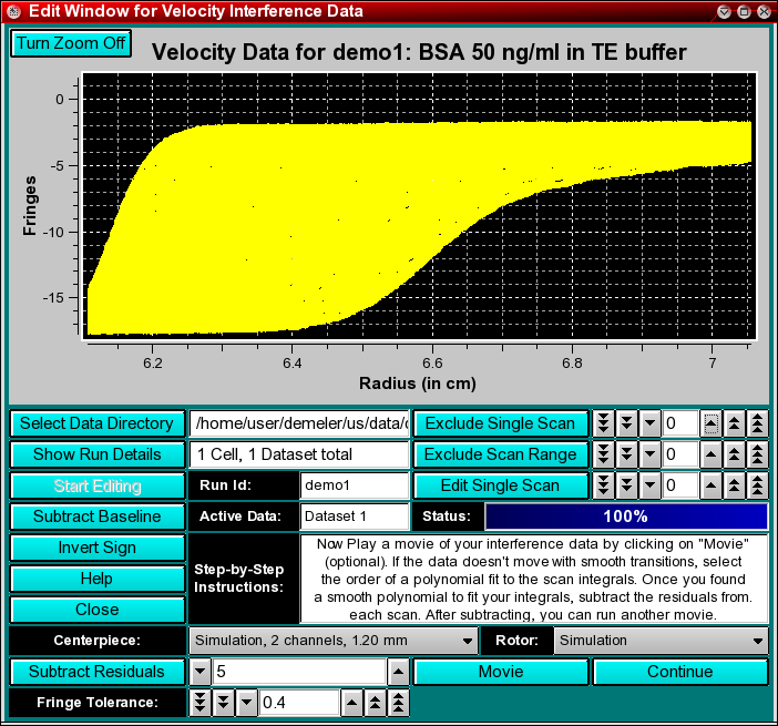
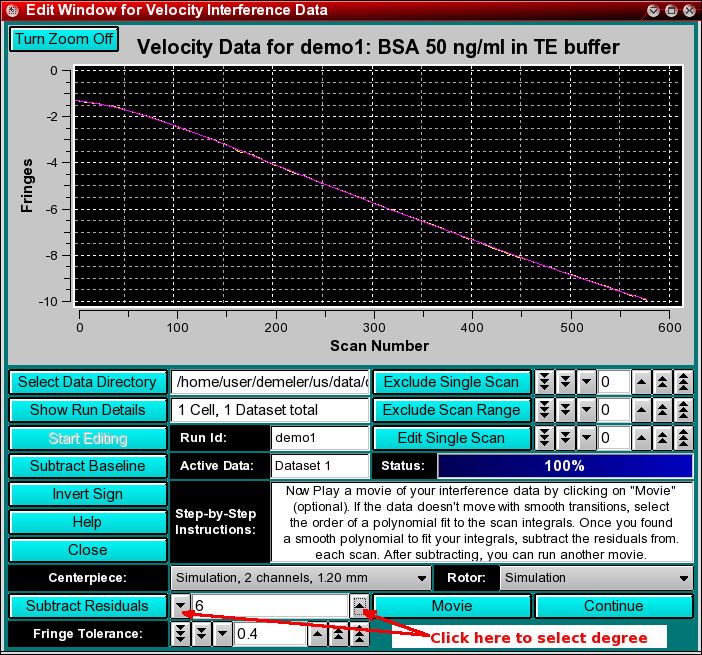
Step 11 (optional): Often, the baseline correction performed in Step 5 is insufficient, since it is subject to averaging in an area of the scan that is often plagued by considerable noise. To determine if the baseline corrections are sufficient, play a movie of the data by clicking on the "Movie" button. If the scans appear to jitter in the movie, it may help to fine-tune the baseline corrections for each scan. UltraScan includes a unique algorithm to substantially improve the baseline offset correction. It is based on the idea that all concentration changes in the cell occur slowly over time and that the function of scan integrals is smooth. While the function is not known exactly (it is dependent on the radial dilution, which depends on the distribution of s values and the diffusion of each component present in the cell, as well as the radial limits of the selected data), it is possible to model the integral function with a smooth function such as a polynomial of nth degree.

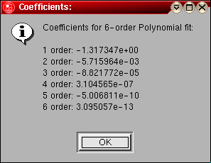
In order to determine which order polynomial best fits the integral function, click on the counter button to select increasing polynomial orders. The fit will be shown in the plotting panel, and the value of the coefficients will be shown in a text dialogue. Use the smallest possible order that fits well. Once the best order fit has been determined, the residuals of the fit describe the baseline offsets that need to be corrected. They can be subtracted by clicking on the "Subtract Residuals" button, which should now be highlighted.

Step 12 (optional): To verify that the data has been properly corrected, you can now play the movie again, the jitter should have disappeared. You can replay the movie multiple times, if desired. Click on the "Continue" Button to proceed with the editing.

Step 13 (optional): After the baseline offsets have been corrected, you can now correct for time invariant baseline contributions by subtracting a baseline scan from all data scans. In order to select an appropriate data scan, click on the "Subtract Baseline" button in the main editing screen. A file dialogue will be shown and allow you to select the correct baseline data file. Double click on the file name and the data will be subtracted from all scans. Typically, you would want to pick and early scan (scan 1 or 2), because it will have the least amount boundary formed and have the longest constant plateau region.

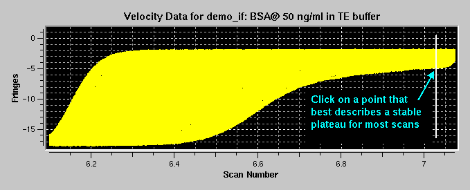
Step 14: Now the corrected and aligned interference data will be shown in the plotting panel and you have to define a plateau interference for all scans by clicking with the mouse at the appropriate point in the cell. Simply pick at a point that defines a stable plateau for most of the scans in the plot. Even if some scans clearly do not meet the criteria of a stable plateau, certain methods will give the appropriate diagnostics (van Holde - Weischet method) and allow you to exclude those scans from the analysis, while other methods (finite-element and other whole boundary fitting methods) can incorporate those scans without a stable plateau into the analysis. After clicking, the program will average a few points to the left and to the right of the point you clicked to arrive at a value for the plateau interference of each scan. Please also refer to the van Holde - Weischet tutorial's section on data editing.

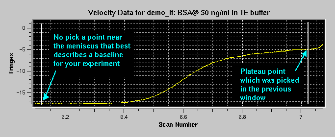
Step 15: The last step in the analysis is the definition for the baseline. After defining the plateau interferences for each scan, the last scan will be displayed, because it will have the most pronounced baseline. Find a point at which the baseline interference is constant and click on it. The program will average a few points to the left and to the right of the point you clicked to arrive at a value for the baseline interference.

Now the data for the first dataset is edited and the program will automatically cycle to the next dataset by returning to the main editing window and updating the progress bar to indicate the status of file loading. Repeat Steps 4 - 14 for all datasets in the run. When all datasets are edited, the program will return with a message window indicating that all scans have been edited and the data has been written to a binary file.