"Manual"

Finite Element Simulations:

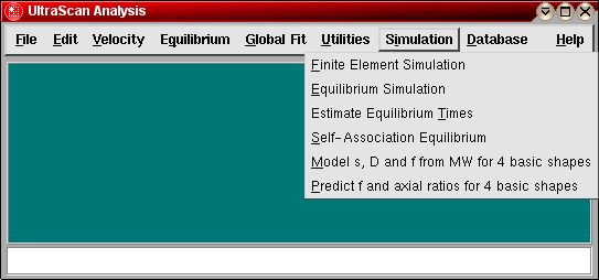
The Finite Element Simulation module can be started from the Simulation Menu in the Main Menu.

General Purpose:

This program can be used to simulate sedimentation velocity and sedimentation approach to equilibrium experiments with the finite element method. You can choose from several models and define all pertinent model parameters such as sedimentation and diffusion coefficients, partial concentration, concentration dependency parameters as well as equilibrium constants for equilibrating systems. The run parameters can be set to control speed, duration of the experiment, presence and extent of time invariant and gaussian distributed noise, scan numbers and frequency, loading concentration and volume as well as cell dimensions. Finite element discretization stepsizes can also be adjusted. The simulated data can then be saved in UltraScan or in the ASCII Beckman XL-A data acquisition format for import into another spreadsheet format, or analysis with various analysis methods. The purpose of the simulation routine is twofold:

1. Allow the researcher to model a velocity or equilibrium experiment based on prior knowledge about the components in the system, so run parameters such as rotor speed and time can be optimized for a particular experiment

2. to serve as an educational module for graduate level courses teaching theory and application of sedimentation analysis.

When using the program to simulate experimental data to determine optimal run conditions, approximate parameters such as molecular weight or stoichiometry are often know. This knowledge can be used to estimate sedimentation and diffusion coefficients with the module for modeling "s", "D" and "f" from molecular weight for 4 basic shapes. After optimal run conditions have been determined, they can be applied to the actual experiment to minimize loss of expensive samples due to misconfigured XL-A/I settings.

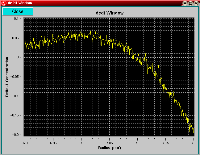
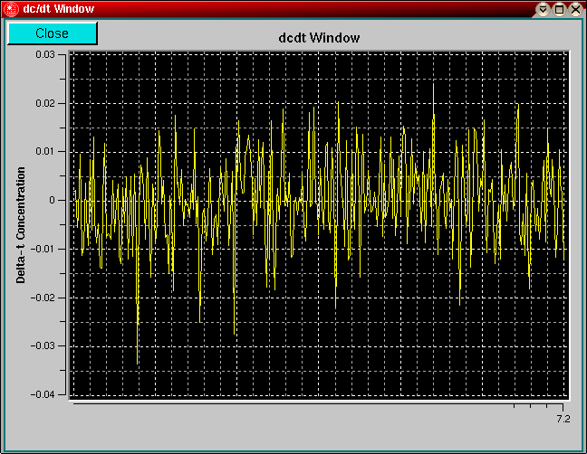
The program can also be used in conjunction with the Equilibrium Speed Estimator to simulate approach to equilibrium experiments. By monitoring the dcdt window, it is possible to determine when further change in concentration is lost in noise and you can effectively tell the time by which equilibrium has been reached (see below).

Model Selection:

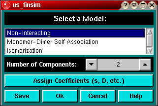
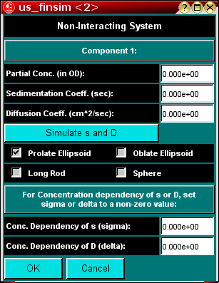
The first step in simulating a sedimentation run is to define a model. This is accomplished by pressing the "Create New Model" button. This will display the Model Selection Dialogue. Select a model from the list. For the non-interacting model you can define the number of components to be modeled with the system. There is no limit to the number of components that can be modeled with this program. After selecting the appropriate model, click on the "Assign Coefficients (s, D, etc)" button to assign values to the model's parameter list.

If you chose a non-interacting system, you will be prompted with a dialogue for entering partial concentration, "s", "D" and concentration dependency parameters sigma and delta. If you have selected to model more than one component, clicking on the "Next" button will cycle through the list of selected components, presenting coefficient dialogues for each component. After entering the last component's parameters, click on the "OK" button to be returned to the Model Selection dialogue.

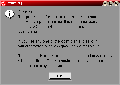
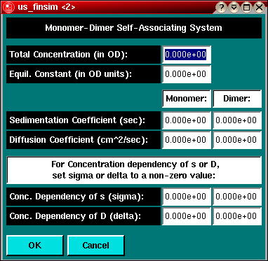
If you choose an equilibrating system, an information message will be displayed informing you that one of the four possible parameters "s" and "D" can be left blank (assigned to zero) because of the molecular weight constraints for the second component. The Svedberg relationship allows three parameters to be specified, while the fourth can then be automatically calculated. The coefficient dialogue for equilibrating systems will display a single screen for both components, While it is possible to assign values for all parameters, you should always leave one of the four parameters set to zero so it can be more accurately assigned by the program itself.

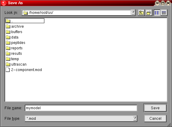
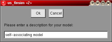
After entering all model parameters, you have the opportunity to save the newly defined model. A file dialogue will appear which allows you to save the model to a file. You will be prompted to enter a short description for your model to facilitate later identification. Once saved, the model can be retrieved at a later time with the "Load existing Model" button from the main finite element simulation panel.

Selection of Run Conditions:

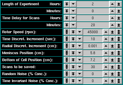
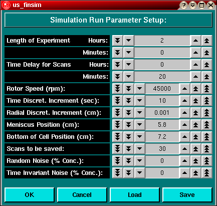
To continue, you click on the "OK" button of the model definition dialogue. You now have the opportunity to enter all relevant run parameters into the run control dialogue. The following run properties can be defined:

Run Duration - the length in hours and minutes of the experiments Time Delay for Scans - the time in hours and minutes before the first scan is recorded. This is similar to the Beckman Data Acquisition program which allows you to program time delays with the Scan Methods. Rotor speed - an acceleration period is not considered in this module. Time Discretization Increment - The size of the time increments used in the finite element simulation. The smaller the increment, the more accurate the simulation, especially for faster sedimenting samples. The tradeoff is that smaller time increments require longer computation times. Radial Discretization Increment - The size of the radial increments used in the finite element simulation. The smaller the increment, the more accurate the simulation, This is especially important for steep concentration gradients as are often caused by fast sedimentation and small diffusion coefficients, particularly at the bottom of the cell. There, oscillations of the absorbance may occur as an artifact of the simulation, when the radial increment is too large. The tradeoffs for smaller radial increments are increased memory requirements and longer computation times. Meniscus Position - determined by the bottom of the cell position (below) and the loading volume Bottom of Cell Position - This value will remain fixed for most cases, but can be used to simulate rotor stretching (which has an influence on the bottom of the cell position) and 6-channel centerpiece geomtry. Scans to be saved - the number of scans to be saved. All scans will be equally distributed in time over the duration of the experiment minus the time delay for scanning. Random Noise - Gaussian (normally) distributed noise with a standard deviation in percentage points of the total absorbance (concentration). A different noise distribution will be simulated for each scan. Random noise can be mixed with time invariant noise by giving both non-zero values to simulate both simulaneously. Time Invariant Noise - Gaussian (normally) distributed noise with a standard deviation in percentage points of the total absorbance (concentration). The noise distribution will remain the same for all scans in the run, simulating time-invariant noise. Time-invariant noise can be mixed with random noise by giving both non-zero values to simulate both simulaneously.

You can save any method for a run for later retrieval by clicking on the "Save" button. Previously saved run methods can be retrieved by clicking on the "Load" button. Click on the "OK" button to be returned to the main finite element simulation panel. To cancel changes in this dialogue, click on the "Cancel" button.

Running the Simulation:

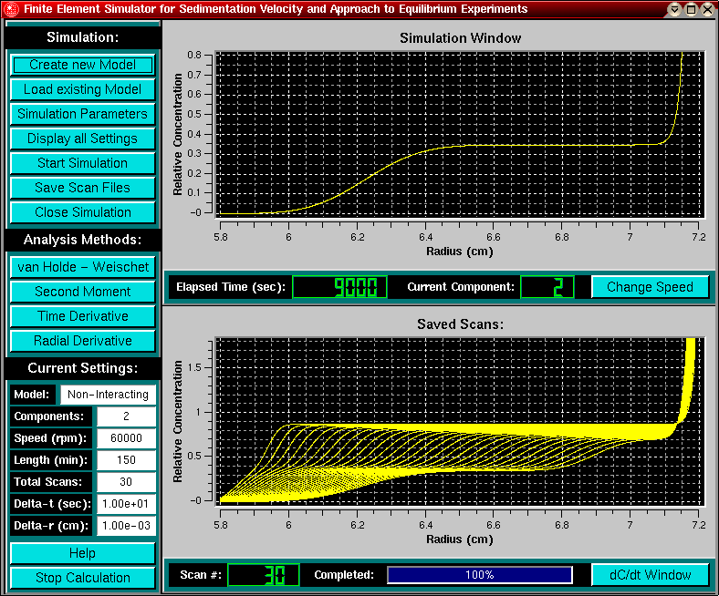
After defining model and run conditions, you are ready to simulate the experiment. Click on the "Start Simulation" button to start the calculation. In the upper panel you will see a movie of the simulation process. In the legend of the upper panel the elapsed time and the component that is being calculated will be shown. For models involving an equilibrium, The letter "E" is displayed to indicate that an interacting equilibrium model is being simulated.

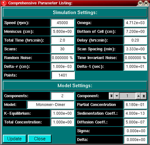
The lower panel will display selected snapshots (scans) from the simulation process, defined by the scan number and delay selected in the run conditions panel. For multi-component non-interacting systems, the scans will not be shown until the last component is being calculated. The scan number and the progress of the overall simulation status is updated in the lower legend. The simulation can be stopped at any time by clicking on the "Stop Calculation" button. A summary of the current run conditions is always shown to the left of the lower plot panel, a comprehensive list of model and run conditions can be displayed by clicking on the "Display all Settings" button.

Running an Approach to Equilibrium Simulation:

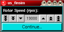
You can simulate approach to equilibrium experiments with this module and use the software to monitor the time it takes to reach equilibrium. When selecting this feature, you need to consider the following settings in the run control dialogue:

1. Only simulate a single component system for this feature - for multi - component systems select the component with the smallest diffusion coefficient, since it will determine the rate-limiting step.
2. Select a short column length, perhaps 3 mm, by setting the meniscus to 6.9 cm, and the bottom of the cell to 7.2 cm. Other centerpiece geometries can be simulated by changing these values.
3. Set the length of the experiment to a sufficiently long time to allow all simulated speeds to come to equilibrium (perhaps 2-3 days)
4. Use the "Model s, D and f from Molecular Weight for 4 basic shapes" module to estimate the sedimentation- and diffusion coefficient for your molecule
5. Use the "Equilibrium Speed Prediction" module to estimate the correct speeds for your experiment
6. Add a little bit of random noise to your experiment to determine a good reference for your signal to noise ratio.
7. Set the number of scans such that the difference in time between scans is at least 2-3 hours.
8. Start the dC/dt window by clicking on the dC/dt Window" button to monitor the approach to equilibrium. When the residuals indicate that the change in concentration from scan to scan is only due to noise, i.e, the residuals are random about zero, you can click on the "Change Speed" button to change the speed to the next higher speed.

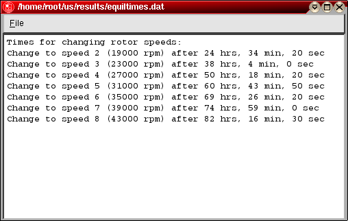
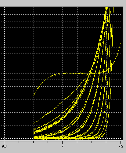
When the simulation is completed, a time window will be shown to indicate how you should set up your XLA to acquire data at the simulated times. This file can be printed out and is available in your results directory under the name "equiltimes.dat". The equilibrium distributions for the simulated speeds will be shown in the data window.

Repeating a Model Simulation with Different Run Condition Settings:

You can simulate the same model under different run conditions without having to redefine your model by simply pressing the "Simulation Parameters" button. This will return you to the Run Parameter Setup Panel, where you can change the run parameters. The run is repeated simply by clicking on the "Start Simulation" button again.

Saving Simulated Data Scans to File:

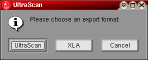
To save the scan files from your simulation for import into a third-party plotting program, click on the "Save Scan Files" button. You will have the option to save the data to an UltraScan compatible "us.v" velocity data file, or to the generic XLA format used in the Beckman data acquisition software.

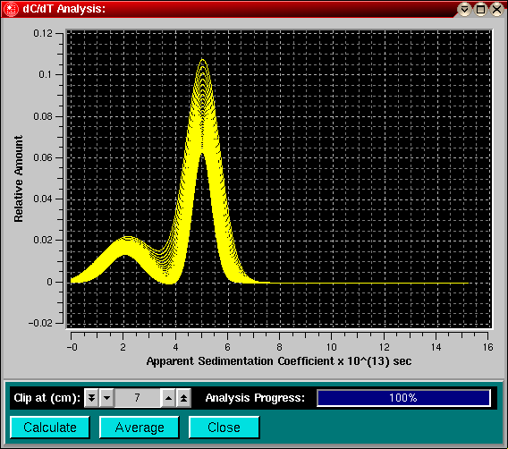
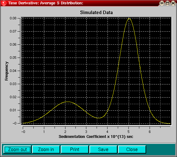
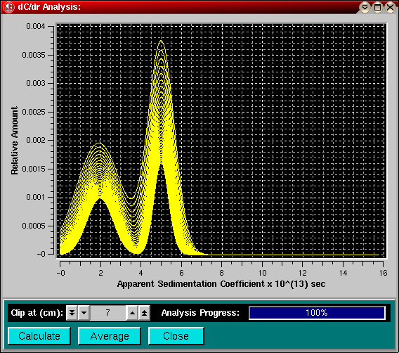
Data Analysis of Simulated Data:

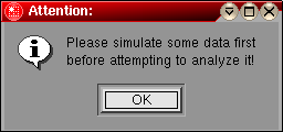
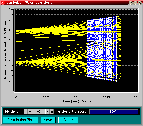
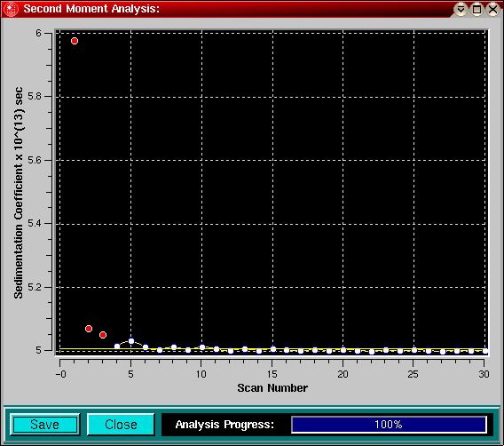
Using the Analysis features of the finite element simulation program it is possible to project the analysis results various methods would yield on a system if it would have been run on the XL-A/I. The analysis modules are particularly useful for teaching the theory of these analysis methods and visualizing the particular strengths of each method. Before any analysis method can be used, it is necessary to actually simulate the data, otherwise an error message will be displayed.

Analysis results from each method can be saved to an ASCII output datafile for import into a third-party plotting program. A description of the file format of this and all other UltraScan output files can be found here. The following analysis methods are available for analyzing your simulated data:

• van Holde - Weischet Analysis: This method is particularly useful to identify and quantify heterogeneity in the sample and to measure concentration dependency of "s". Integral distributions of the van Holde - Weischet data can be constructed to assist in the quantification of the heterogeneity.
• Second Moment Analysis: The Second Moment analysis is useful to detect global changes that occur over the course of the run. These may include degradation, time-dependent aggregation, and pelleting of sample. If the sample has not cleared the meniscus (as defined by 1/2000 of the total absorbance), and error message is displayed, and the plot points corresponding to scans with uncleared meniscus absorbance are printed in red.
• Time Difference - Delta-C/Delta-t Analysis: The Time difference method excels at eliminating time invariant noise, as may be present in interference data or absorbance data with dirty windows. Delta-C/Delta-t scan averages can be displayed by clicking on the "Average" button in the dcdt window.
• Radial Difference - Delta-C/Delta-r Analysis: The radial difference method also provides derivative-domain data, although for most practical purposes the analysis is often compromised by noise in the experimental data. The average of multiple scans can sometimes compensate for some of the noise.

To exit the program, click on the "Close Simulation" button.