
|
|
Manual |
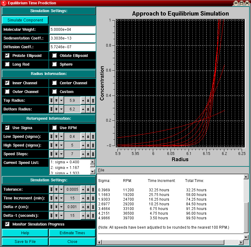
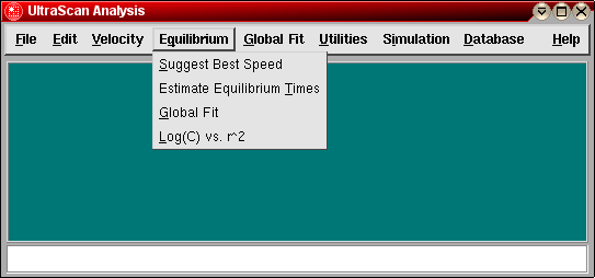
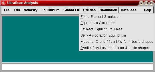
The Equilibrium Time Estimation module can be loaded from the Equilibrium Menu or the Simulation Menu in the Main Menu section of UltraScan.
Whenever you are planning or designing an equilibrium experiment, the question comes up of how long it takes to reach equilibrium at a certain speed. The time it takes depends on several factors:
How to use this module:
When designing an equilibrium experiment, you should plan to acquire equilibria at multiple speeds (4-5 speeds, ranging from sigma=1 - sigma=5, use this program to predict the correct speeds), and therefore it would be nice to estimate before you start the experiment how long it will take to reach equilibrium. Using the finite element simulator programmed in this module, you can predict the time it takes to reach equilibrium for all practical purposes, i.e., the change over time is less than a certain tolerance value. You can then pre-program the speeds into the XLA and are not required to check for equilibrium evertime before you change to the next speed.
When simulating these times, you should simulate a molecule that is sedimenting slightly slower than the actual molecule, perhaps by simulating a system with a larger frictional ratio or larger axial ratio, and perhaps a nonglobular model rather than a spherical model. While the equilibrium times may be longer than needed, at least they won't be too short. In this module you can change the parameters that influence the time it takes to reach equilibrium.
|
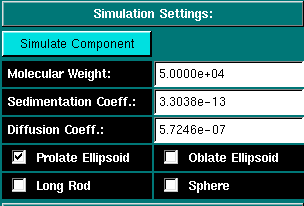
Simulation Settings: Before you can simulate the equilibrium times, you will have to define the molecular parameters for the system to be simulated. Clicking on this button will invoke an UltraScan module used for the prediction of s, D and f from the estimated molecular weight for 4 basic shapes. Once the system is defined in this module, the values will be automatically transferred to the equilibrium times prediction module. The molecular weight of the simulated component. The sedimentation coefficient for the simulated component. The diffusion coefficient for the simulated component. These are the possible models for the selected molecular weight. Selecting the prolate ellipsoid (default) will handle most cases, even spherical molecules with a small time penalty. It is therefore a good default setting. |
|
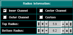
Here you can select the column length and position. You can select from pre-set radii for the 6-channel centerpieces or select custom top and bottom radii for the column. The column height depends on the loading volume and the centerpiece geometry. You can either perform a quick radial scan or determine the radius positions empirically. The longer the column height, the longer the experiment will take to equilibrate. |
|
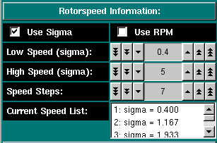
Rotorspeed Settings: Select if you want to enter the speeds in terms of sigma (reduced molecular weight term: [(M * omega^2 * (1 - vbar * rho))/ 2 * R * T]) or by RPM. Either unit will be interconverted. Check this program for appropriate speeds. Select the first speed to be equilibrated Select the last speed to be equilibrated The total number of speeds to be simulated, including the high and low speed. These will be chose linearly spaced between the high and low speed. All selected speeds will be listed here.
|
|
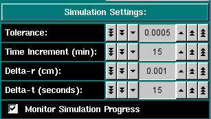
Simulation Settings These settings allow you to control the simulation. This value is the tolerance setting that determines if a scan has reached equilibrium. Successive scans are subtracted from each other and the differences between them are summed up. If the sum is less or equal to this tolerance value, the program will consider the speed equilibrated and automatically proceed to the next speed. For a 3 mm column with 0.001 cm resolution the accuracy of the computer allows about 1.0x10⁻⁵ for the smallest practical tolerance (noise-free data). This is the time between successive scans. The larger the time difference, the coarser is the time determineation, but the more reliable is the time estimation. A good default setting is 15 minutes, to be used with a 5 x 10⁻⁴ tolerance setting. This is the radial resolution used in the finite element analysis and defines the radial discretization step size. A good default value is 0.001 cm, the lowest possible setting in the XLA. This is the time resolution used in the finite element analysis and defines the time discretization step size. A good default value is 15 seconds, since changes over time are rather slow, especially in the end. Show all intermediate scans, otherwise only plot the equilibrium scans. |
|
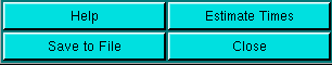
Show this helpfile. Perform the time estimation. This function can only be used after the molecule has been defined. Save the contents of the text dialogue to a file. Same function as selecting "Save" from the file menu. Close the program. |
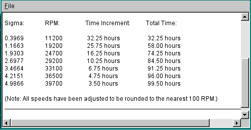
Shown below is the text editor window that will display the incremental and total times for reaching equilibrium:
This document is part of the UltraScan Software Documentation
distribution.
Copyright © notice.
The latest version of this document can always be found at:
Last modified on April 12, 2003.