
|
|
Manual |
| Part 1: Setting up a fitting project | Next: Next: Model Selection |
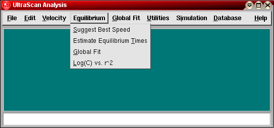
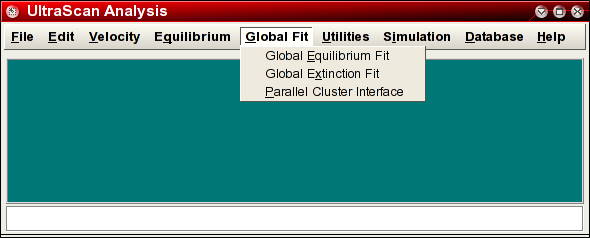
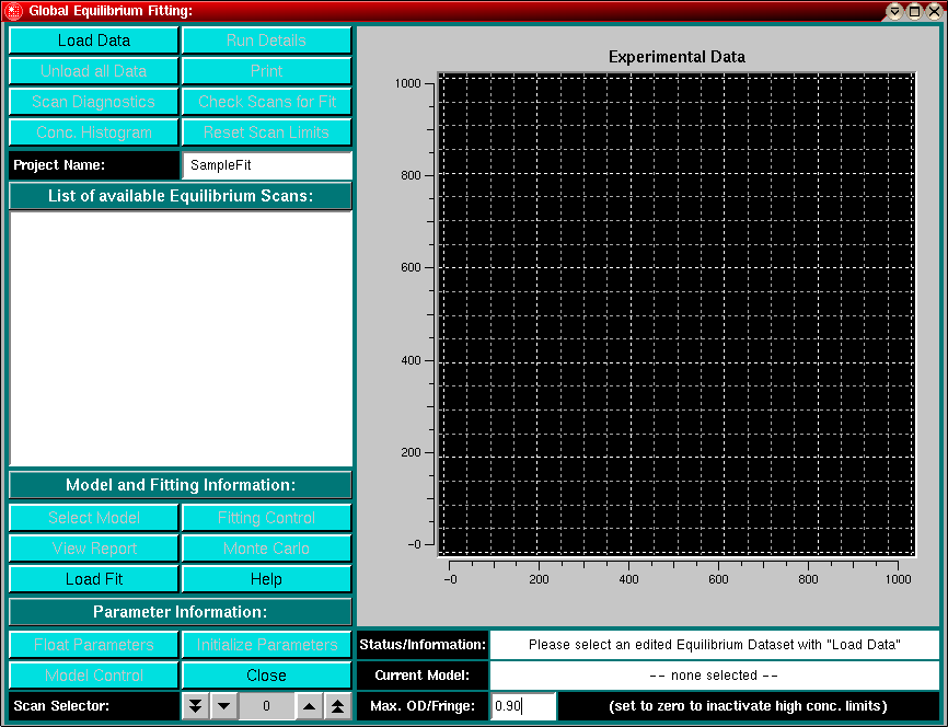
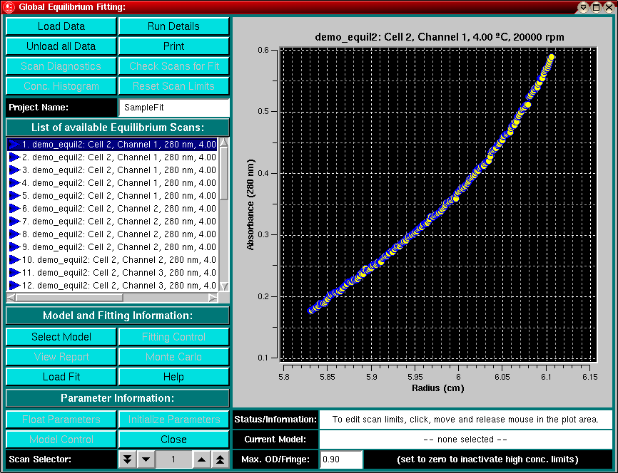
This document describes how to fit your equilibrium data to a global model describing your data by using nonlinear least squares minimization. This is handled with the global equilibrium fitting module of UltraScan. You can start this module from the "Equilibrium" menu under "Global Fit" or from the Global Fit menu. Loading this program will display the global equilibrium control panel. A number of buttons are greyed out, indicating that those functions are not available at this point in the fit.
Importing experimental data:
First, you need to select appropriate datasets for the fit. For any global fit, it is necessary that the data in each individual dataset involves some aspect of the system under investigation which can be represented globally. Typically, for an equilibrium experiment, this would be one or more molecular weights, or the association constants describing the dissociation or association of components, which may be the same or different (self-association vs. hetero-association). Other parameters that may be considered global are the partial specific volumes, which can be determined if the molecular weight of the sample is known beforehand. Should the molecular weight of the sample be determined, the partial specific volume of the molecule needs to be known. Those values can be either determined in an independent measurement, or by estimation from primary sequence. Other parameters are considered local, such as baselines or amplitudes of exponential terms for non-interacting samples.
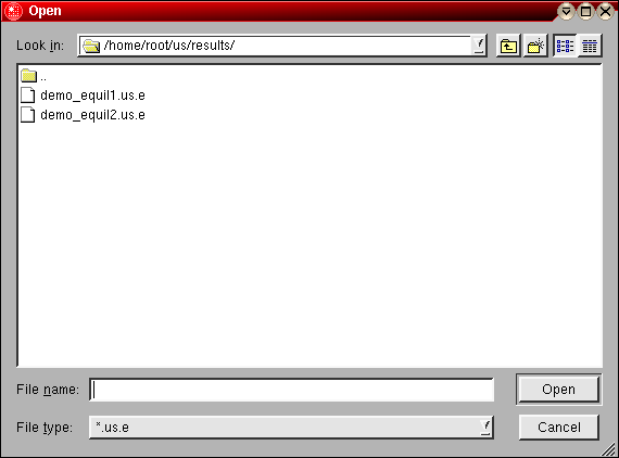
To set up the fit, experimental data needs to be imported. This can be accomplished in one of two ways: First, you can import experimental data by loading an UltraScan equilibrium dataset that has previously been edited with the UltraScan editing module. Second, you can load a previously saved fit, this method is describe in more detail below.
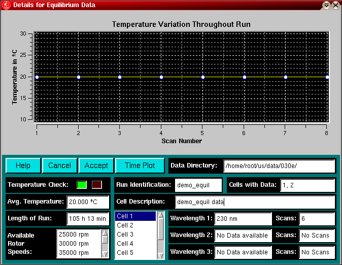
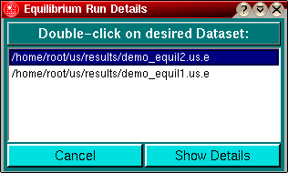
All UltraScan sedimentation equilibrium datasets have the suffix ".us.e". To load edited experimental data, click on the "Load Data" button in the left upper corner of the control panel. Simply select the desired run from the selection of available runs in the dataset loading dialog. Once loaded, the Run Details will be shown. Click on the "Accept" or "Cancel" button, and you will be returned to the main analysis window, now with the first dataset loaded, and the first scan displayed in the plot area. For information on how to edit equilibrium data, please check here.
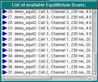
The global equilibrium fitting program considers equilibrium fits as "Projects", which can consist out of more than one experimental dataset, or out of several combined datasets. There is no program limit to the number of datascans that can be imported. You can import several edited runs, which in themselves consist of multiple scans. The datasets do not have to be (and should not be) all at the same speed, temperature, concentration, or wavelength, since a variation in those parameters improves the signal spectrum for the fit. Moreover, these parameters can be adjusted and compensated for individually. (Please check the Global Nonlinear Least Squares Equilibrium Tutorial for details on how to design good experiments and select appropriate data).
After loading one or more datasets, several buttons will become activated and you will be able to perform additional functions. The first scan will be displayed in the plot area, and the descriptions of the available scans from the selected run will be shown in the listbox for all available equilibrium scans.
Loading data activates the following additional functions:
The second way of importing data is to load a fit from a previous
fitting session. This is accomplished by clicking on the "Load Fit"
button. All settings from the previous fit will then be restored in a complete
memory copy of the memory state when the fit was saved. It will restore
all scan limits, fitting parameters, run parameters and all scans and
their settings from the point where they were saved. The data can then
be used for further refinement or to change to a different model. Each step
is explained in the following documents.
Naming the Project:
Each fit is considered a project, which may consist out of more than one
equilibrium run. In order to avoid naming conflicts, the name of the project
should be different than the name of the run. Descriptive project names are
recommended, however, spaces in the project name should be avoided. You should
rename your project from the default "SampleFit" to something that you can
remember by entering a new name in the "Project Name:"
field.
Selecting a Maximum Optical Density
Absorbance scans will suffer from nonlinearity above a certain optical density.
Therefore it is prudent to only consider data within an absorbance range that
has been verified to produce linear results. These limits may be different
for different wavelength. Check your instrument to determine within which
range your data is reliable. You can change the absorption cutoff limit by
entering it into the Max. OD/Fringe: field. A value of
zero inactivates automatic high concentration limits, however, you will be
able to manually adjust limits on each scan (discussed in
Section 3). The default setting for this parameter is 0.9 OD.
Other Functions:
| Setting up a Fitting Project | Next: Model Selection |
This document is part of the UltraScan Software Documentation
distribution.
Copyright © notice.
The latest version of this document can always be found at:
Last modified on January 12, 2003.