Manual

Finite Element Analysis - Model Control Window:

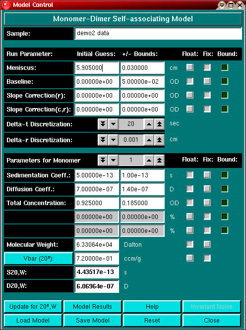
The model control window allows you to enter initial guesses for the fitting process, control linear constraints and determine which parameters should be floated during the fitting process and which should stay fixed. In this window you can also control the simulation accuracy by changing the discretization stepsize. During the fitting process the guesses will be updated by the nonlinear least squares fitting routine.

Entering Initial Guesses:

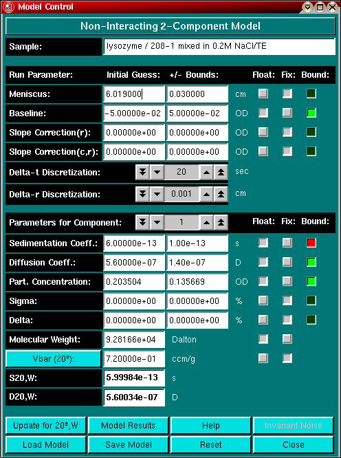
First, you need to enter initial guesses for the various parameters. Some parameters will already have an approximated value listed, which may or may not suffice for fitting. Generally, the closer the value of the initial guess is to the true value, the faster the fitting process will converge. Estimates such as the meniscus position, the total concentration and baseline absorbance will be taken from the editing routine. For non-interacting multi-component systems, it is assumed that the total absorbance is equally distributed over each component. Modify the partial concentration for each component according the integral distribution of the van Holde - Weischet method, where you can define groups to obtain initial guesses for the sedimentation coefficient and the partial concentration. By clicking on the Parameters for Component: counter, you can navigate between the parameter settings of all components defined in the model. If you selected the "Fixed Molecular Weight Distribution" model, you can directly import the saved van Holde - Weischet model into the model control window by clicking on "Load Model". For more information on this option, please check the information on the fixed molecular weight distribution model and refer to the Group Definition function in the van Holde - Weischet analysis.

Parameters such as Slope Correction of "r" and "C,r", Sigma and Delta (concentration dependency parameters) are initialized to zero. When set to zero, these parameter will not have any effect on the fit. These four parameters are the only parameters that can be excluded from the fitting model by being set to zero, all other parameters need to have a finite value. Of course, the baseline absorbance value can be zero, but that does not exclude it from the model.

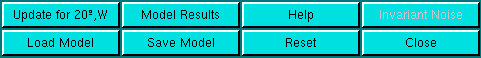
Enter the parameters for s and D and adjust the partial concentration, if necessary. You can use the "Calculate Protein MW and vbar" utility by clicking on the "Vbar(20^oC)" button to set a partial specific volume, or alternatively type the value in by hand. Be sure to enter the value corrected for 20^oC, the program will automatically correct for temperature as described in Cohn & Edsall (Proteins, Amino Acids and Peptides as Ions and Dipolar Ions. New York. Reinhold, 1943.). If you have set the buffer conditions in the finite element panel, hydrodynamic corrections based on buffer conditions will automatically be applied when you click on the "Update for 20^oC,W" button and a molecular weight will be calculated from the corrected S- and D-values. Also, a temperature and buffer corrected S- and D-value will be displayed in the s20,W and D20,W field. Each time you change either the buffer values or the partial specific volume, you have to click on the "Update for 20^oC,W" button to make sure the values are properly updated.

If your model contains more than one component, select each component by clicking on the counter Parameters for Component:. Please make sure to enter the uncorrected values for s and D. If you only have the corrected values available, adjust the value for s and D until the corrected value matches the value shown in the S 20,W and D 20,W field. A small inaccuracy is quite tolerable here and can be compensated for by the finite element fitting process, however, the closer the value to the true value, the faster the solution will converge.

For the Monomer-Dimer model, the molecular weight of the dimer is constrained by the molecular weight of the first component (by mass action and the Svedberg relationship). This means that the second component's molecular weight and diffusion coefficient cannot be changed manually. Also, the concentration dependency parameters are greyed out, since fitting these parameters in multicomponent systems is not justified, unless multiple experiments can be fitted simultaneously. This functionality will be added at a later point in the Beowulf version of UltraScan. The association constant for this model is fitted in OD concentration units, if you prefer molar^-1 units, you will need to convert the result, which requires knowledge of the molar extinction coefficient.

Setting Bounds:

The program employs the DuD (Doesn't use Derivatives) non-linear least squares fitting algorithm to minimize the square of the residuals. This algorithm requires a matrix of initial guesses which is orthogonalized by offsetting the diagonal element by the range of possible values. To assure that this matrix is non-singular, the value of the range needs to span the solution space. You have control over this process by entering bounds that are added and subtracted from the initial guess to form the initial guess matrix. In practice, it is recommended to let each parameter vary 10% - 20% of the total amount of the parameter. The value of the bounds should also be determined by the confidence you have in each initial guess. For example, if you fit for the meniscus position, you will probably not need to let the meniscus position vary by more than 2% - 3%, since this value can be determined with great confidence from the edited data. However, diffusion coefficient estimates are much less precise, and require a larger range for the bounds. Of course, you only need to enter bounds for parameters that are set to float. Fixed parameters do not require a range setting and range settings for fixed parameters will have no effect. Make sure to enter reasonable bounds (i.e., no negative diffusion coefficients, or negative concentrations, etc) and make sure not to forget to enter the bounds for each component of your model.

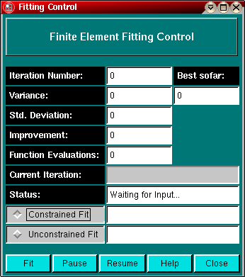
Constrained and unconstrained fits:

In the fitting control dialog you can select to use linear constraints for your fit. If the fit is constrained, the control window will indicate by using red labels if a parameter is attempting to go outside of bounds. If parameters are adjusted within the linear bounds by the fitting routine, the label will switch to green. If a parameter consistently is marked with a red label, you should examine the bounds set before fitting. Linear constraints can help you fit a dataset by preventing nonsensical parameter values occuring during a fit.

Floating or Fixing?

The general rule is to fix as many parameters as possible and to constrain the fit as much as possible. Oftentimes, you already know the molecular weight of the component. If you enter and fix the molecular weight, the s/D ratio will be calculated according to the Svedberg relationship. When fixing the molecular weight, you have two options: you can let the partial specific volume float, or the diffusion coefficient. If you are not sure of the molecular weight but have a good idea about the partial specific volume of a sample, it is often sufficient to float the baseline, the partial concentration as well as s and D. Don't forget to enter the proper floating/fixing setting for all components in your model.

Sloping Baselines:

If your data has optical flaws, such as a sloping baseline, you can compensate for this error by setting the slope correction to a small, nonzero value (on the order of 1x10^-2) and floating it. Use positive values for increasing plateaus, and negative values for decreasing plateaus. A second order slope correction approximation can be achieved with "Slope Correction (C,r)", which is proportional to C and linear with r.

Discretization Intervals:

Using the Delta-t and Delta-r discretization counters, you can adjust the stepsize for the time and radius discretization used in the finite element solution. The smaller the step size, the more accurate the solution, but the more time or memory it will take to complete the calculation. For the radius, a 1x10^-3 cm setting is usually sufficient. For very small diffusion coefficients or fast run speeds, a smaller setting may be more appropriate. If you get errors at the bottom of the cell (oscillations of the absorbance), decrease the radial discretization to about 5x10^-4 cm. The time discretization doesn't appear to have a lot of influence on the accuracy of the solution, as long as the change of the concentration gradient isn't too rapid. For initial fits, a 10-20 sec setting is generally quite appropriate, for slow sedimenting material or approach-to-equilibrium experiments even a larger setting is appropriate. Once the fit has converged, the final solution can still be refined with a smaller discretization stepsize. All parameters, with the exception of the fixed/floating setting, and the discretization settings, may be changed and adjusted manually during the fit. For more information, see the Fitting Control help file.

Model Window Control Panel:

• Update for 20^o,W: Takes current settings for temperature, buffer and partial specific volume and corrects s and D for values at 20^oC and water. Also updates the resulting molecular weight.
• Model Results: Take current values for s and D and apply theoretical models to calculate molecular dimensions. The models calculated include a sphere, a prolate ellipsoid, an oblate ellipsoid and a solid rod. Please bear in mind that these models are hypothetical only! For more information, consult the Finite Element Result Interpretation Manual.
• Help: This help file
• Invariant Noise: Model time invariant and radially invariant noise (not implemented yet)
• Load Model: Load a predefined model from disk. The model must match the current model selection
• Save Model: Save current model settings to a disk file for later retrieval
• Reset: Reset parameter initial guesses with default guesses
• Close: Close window

Please read the Finite Element Tutorial for more tips on optimal analysis strategies.